Machine Learning- Gender Recognition

INTRODUCTION

Human ear has an excellent mechanism of perceiving the voice. It distinguishes the voice based on factors such as the loudness, frequency, the pitch and the resonating frequency. We are going to test several classification algorithms mentioned above on the voice dataset provided by kaggle.com [1]. The dataset consists of 3,168 recorded voice samples, collected from male and female speakers. 20 acoustic properties of each voice are measured and included within the first 20 columns of the CSV file, whereas the genders of samples are placed at the last column. The purpose of our work is to figure out whether the voice belongs to male or female by using various statistical analysis and machine learning algorithms. We will also be analyzing and using various data preprocessing techniques to make the data more clean that can be generalized easily to apply the various Machine Learning algorithms to predict the gender of the sample based on the data samples.

PROBLEM

A human ear can distinguish between a male and female voice easily. If we want to teach a machine to do the same then what features of a voice would the machine require to classify ? The voice of an adult male can range between 85 to 180 Hz and that of adult female ranges between 165 to 255 Hz[2]. We can see that although the frequency ranges differ quite a lot, there is a mid range where they seem to overlay. This is why differentiating voices only on the basis of frequency is challenging and the purpose of our work is to figure out whether the voice belongs to male or female by the use of various ML techniques based on the given features in our dataset.

Another interesting problem we have thought from this dataset is predicting the pitch or the mean frequency of the instance using the various regression algorithms, in this case we have a regression problem instead of classification problem as the above one.

FEATURES

Features in the dataset were obtained from voice samples which are pre-processed by acoustic analysis in R using the seewave and tuneR packages they are as follows:

1. Mean frequency (meanfreq) Mean normalized frequency of the spectrum of the audio signal, measured in kHz.

2. Standard Deviation of Frequency (sd) Standard deviation measures the amount of variation or dispersion of data values. A low standard deviation indicates that the values are more closer to the mean, whereas a high standard deviation indicates that the values are more spread out.

3. Median Frequency (median) Median frequency is the middle value of a dataset and is measured in kHz.

4. First Quantile (Q25) Quantiles are the points dividing range of probability distribution into contiguous intervals with equal probabilities. It is the data value when the standard distribution goes beyond the first threshold. It is measured in kHz.

5. Third Quantile (Q75) Similar to the first quartile, the third quantile is a data point when the standard deviation reaches the one third of the highest in the range. It is measured in kHz.

6. Interquartile Range (IQR) Interquartile Range is the difference between the first (lower) and the third (upper) quartile and is measured in KHz. It is a measure of statistical dispersion.

7. Skewness (skew) Skewness is a measure of the asymmetry of the probability distribution of a real-valued random variable about its mean. The skewness value can be positive or negative, or even undefined. Skew can be thought to refer to the direction opposite to that where curve appears to be leaning.

8. Kurtosis (kurt) Kurtosis is a measure of the ”tailedness” of the probability distribution of a real-valued random variable.Similar to skewness, kurtosis is a descriptor of the shape of a probability distribution and just as for skewness,there are different ways of quantifying it for a theoretical distribution and corresponding ways of estimating it from a sample from a population.

9. Spectral Entropy (sp.ent) In general, entropy is nothing more than the measure of amount of disorders in a system. Spectrum Entropy tells us how different the distribution of energy is in the system. High value of spectral entropy indicates the existence of a constant similarity of energy (small variations). Low value of spectral entropy indicates high variances and irregularity.

10. Spectral Flatness (sfm) Spectral Flatness is a measure used in digital signal processing to characterize an audio spectrum. It is also known as Wiener entropy. It is typically measured in decibels and provides a way to quantify how noise-like a sound is, as opposed to being tone-like.

11. Mode frequency (mode) Mode frequency is the one occurring most in the entire dataset.

12. Frequency centroid (centroid) The frequency centroid is a measure used in digital signal processing to characterize a spectrum. It indicates where the ”center of mass” of the spectrum is. Perceptually, it has a robust connection with the impression of ”brightness” of a sound.

13. Mean Frequency (meanfun) Average of fundamental frequency measured across acoustic signal.

14. Minimum frequency (minfun) Minimum fundamental frequency measured across acoustic signal.

15. Maximum frequency (maxfun) Maximum fundamental frequency measured across acoustic signal.

16. Average dominant frequency (meandom) Average of dominant frequency measured across acoustic signal.

17. Minimum dominant frequency (mindom) Minimum of dominant frequency measured across acoustic signal.

18. Maximum dominant frequency (maxdom) Maximum of dominant frequency measured across acoustic signal.

19. Range of dominant frequency (dfrange) Range of dominant frequency measured across acoustic signal.

20. Modulation index (modindx) Calculated as the accumulated absolute difference between adjacent measurements of fundamental frequencies divided by the frequency range. It describes by how much the modulated variable of the carrier signal varies around its unmodulated level.

DATA & PREPROCESSING

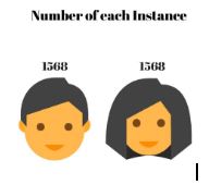
From Fig 1, we can see that the number of female and male samples are the same, indicating that there is no unbalanced problem in our dataset.

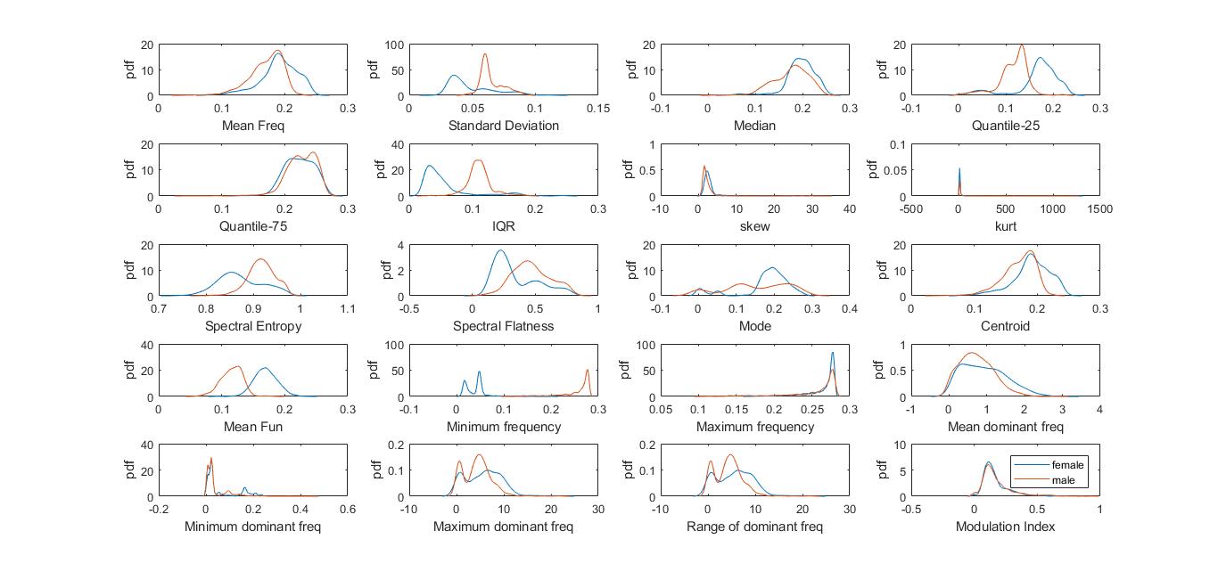
In Fig 2.we have plotted the PDF function of every male and female data points present in the database for a particular feature against each other. We can observe that there is more overlap region in the distribution plots of features like centroid, meanfreq, minfun, modindx and Q75. In addition, the distribution plots of features like IQR, meanfun, mode, Q25, sd have less overlap region i.e the values are more scattered[4].The features having less overlap region are more important features since they show greater variation in data which will be of great use in predicting the gender of the given instance. We can also analyze that as the overlap region between male & female instance of a particular feature increases the redundancy of the data from that particular feature also increases,this point is also supported by the analysis done further in the project.

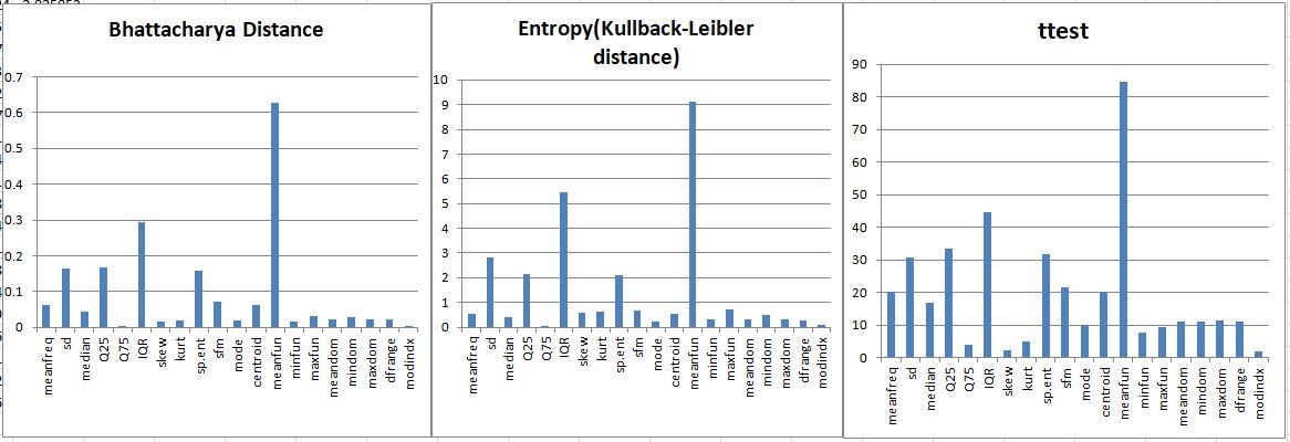
The feature importance is shown in Fig 3. is extracted using three different methods i.e Bhattacharyya distance,Entropy,t-test.

Bhattacharyya Distance

Bhattacharyya Distance measures the similarity of two discrete or continuous probability distributions. Bhattacharyya coefficient is a measure of the amount of overlap between two statistical samples or populations.Higher the value of Bhattacharyya Distance less is the overlap region[7].It can be seen from the plot above that meanfun, IQR, Q25 are the three most significant attributes in the dataset. The lower value of the Bhattacharyya distance indicates the data quite overlap each other while the higher value of it indicates that the pdf for male and female are quite apart and is an important features for classification

Kullback –Leibler divergence

This is a measure of how one probability distribution diverges from a second probability distribution.It is widely used in characterizing the relative (Shannon) entropy in information systems, randomness in continuous time-series, etc. A Kullback–Leibler divergence of 0 indicates that we can expect similar behavior of two different distributions, while a Kullback–Leibler divergence of 1 indicates that the two distributions behave in such a different manner[8].

T tests

In our binary classification problem,each sample is classified either into class C1 or class C2. t-Statistics[11] helps us to evaluate that whether the values of a particular feature for class C1 is significantly different from values of same feature for class C2. If this holds, then the feature can help us to better differentiate our data.

All the three test used here gives us similar results. Based on this, the most important 5 features of our dataset are selected

• Mean Frequency
• Inter-Quantile Range
• Q25
• Standard Deviation
• Spectral Entropy

CORRELATION

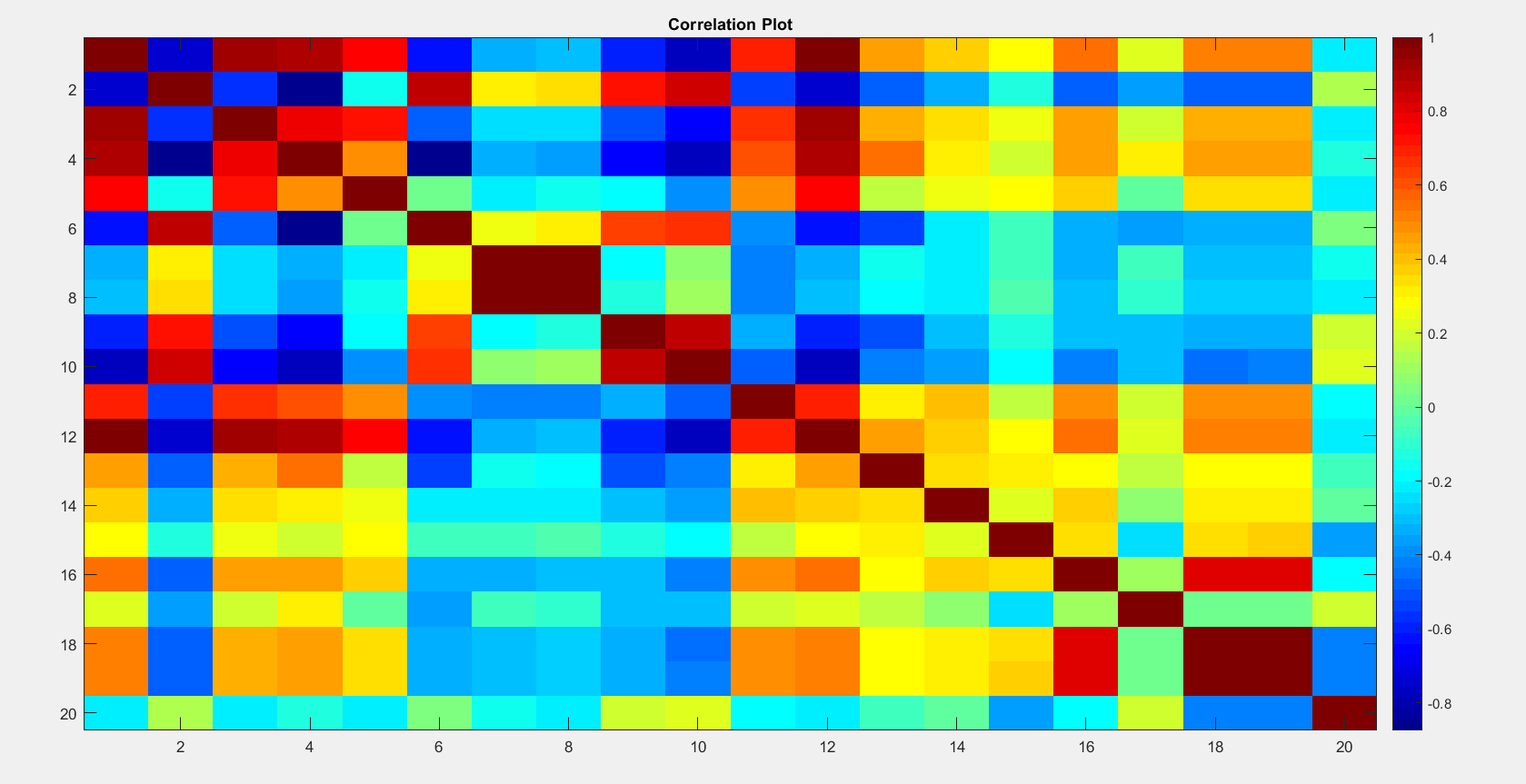
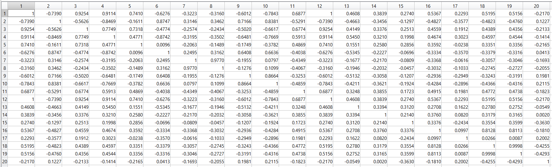
The above figures shows that some of the variables have very high correlation which is more than 0.8 (Fig 4), such as meanfreq, centroid, Q25, standard deviation, median, spectral flatness, maximum dominant frequency, range of dominant frequency and skew. Features having high correlation gives redundant data and hence can be eliminated without much loss of information. Out of two highly related features, the one having higher variance with other features is eliminated.Due to the high correlation among variables, we used PCA to reduce the dimensions.

STATISTICAL MEASURES

We have performed various statistical techniques on our raw dataset and observed that the range of features are quite different. Some features such as feature-7 has a very large range, This will cause problem while using distance based techniques due to non-uniformity. Therefore scaling of features is need of the hour, and also for applying PCA one has to do mean normalization and scaling.

NORMALIZATION

Some machine learning algorithms based on the gradient descent or on distance measures like KNN are quite sensitive to the scale of the numeric values provided. Consequently, in order for the algorithm to converge faster or to provide a more exact solution, rescaling the distribution is necessary. Rescaling mutates the range of the values of the features and can affect variance, too. Hence Normalization becomes a very important step in data preprocessing. These can be done by using various statistical standardization like z-score normalization,min-max transformation, division by max value etc.

• Z-score normalization It is to center the mean to zero (by subtracting the mean) and then divide the result by the standard deviation.

• The min-max transformation This is to remove the minimum value of the feature and then divide by the range (maximum value - minimum value). This act rescales all the values between 0 to 1. It’s preferred to standardization when the original standard deviation is too small original values are too near or when you want to preserve the zero values in a sparse matrix.

• Division by max value It is basically dividing the whole feature dataset by its maximum value this process also rescales all the value between 0 to 1.

After applying all the above stated normalization techniques we have used the new normalized from each of the three techniques on the ML algorithm and found that all the mentioned techniques are giving equivalent results while Z-score normalization being slightly better off than rest.

OUTLIERS

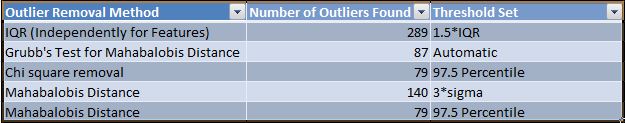
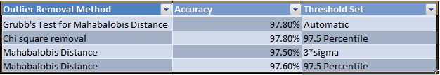
An outlier is an observation that diverges from an overall pattern on a dataset. We know that Machine learning algorithms are very sensitive to the range and distribution of these values. Here outliers can play spoilsport and mislead the training process resulting in longer training times, less accurate models and ultimately poorer results. Hence it becomes necessary for us to remove outliers. They are of two kinds: Univariate and multivariate. Univariate outliers can be found when looking at a distribution of values in a single feature space. Multivariate outliers can be found in a n-dimensional space (of n-features). We have multivariate data here. Many univariate outlier detection methods can be extended to handle multivariate data. The central idea is to transform the multivariate outlier detection task into a univariate outlier detection problem. Here we have used Mahalanobis distance and chi-square statistic for multivariate outlier detection. The method gives a univariate variable, and thus univariate tests such as Grubb’s test,interquartile range method,3-sigma method can be applied to this measure.

Mahalanobis distance [5][6]

It is a measure of the distance between a point P and a distribution D, It is a multi-dimensional generalization of the idea of measuring how many standard deviations away P is from the mean of D. This distance is zero if P is at the mean of D, and grows as P moves away from the mean along each principal component axis, it measures the number of standard deviations from P to the mean of D. Mahalanobis distance is unitless and scale-invariant, and takes into account the correlations of the data set. Using this method we get a univariate in which for checking outlier we have set the threshold as 97.5% Quantile of chi-square distribution[12].

chi-square test [6]

It is a statistical test of independence to determine the dependency of two variables[13]. From the definition, of chi-square we can easily deduce the application of chi-square technique in feature selection. We have a target variable from the dataset of a feature and mean variable being the mean of the data points of the feature from which we select target variable. Now, we calculate chi-square statistics between every mean variable and the target variable and observe the existence of a relationship between the mean variables and the target[14]. Larger the chi-square statistic, the target/object is an outlier in our case above 97.5%[15]

Grubbs’ Test [6]

It is maximum normalized residual test or extreme studentized deviate test, is a statistical test used to detect outliers in a univariate data set of a normally distributed population. Here we used the grubbs’ test by converting the multivariate data into a univariate data by mahalanobis distance and then used it on grub’s test. Grubbs’ test detects one outlier at a time. This method will continue to run until all the outliers are removed from the dataset. Grubbs’ test is defined for the hypothesis:

Interquartile range method

We process the data using the above method, here we observe that if the value of the given data is less than the value of Q25-1.5IQR or greater than that of Q75+1.5IQR, then we classify it as an outlier[6]. Where Q25 is 1st quartile, Q75 is the 3rd quartile and IQR is interquartile range and the outliers are detected.

3 sigma method

In this we basically observe that if the data value is greater or lesser than the distance from the mean of the features to three times its standard deviation value,then it is classified as a outlier.

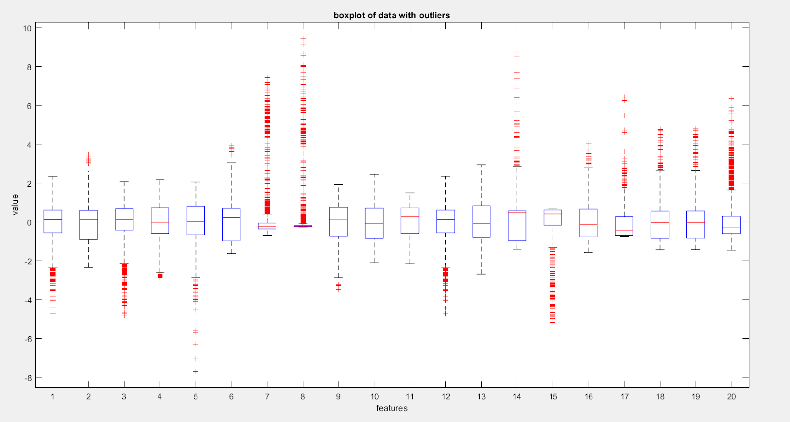
Here on the each box, the central mark indicates the median, and the bottom and top edges of the box indicate the 25th and 75th percentiles, respectively. The whiskers extend to the most extreme data points not considered outliers, and the outliers are plotted using the ‘+’ symbol. As shown in the Figure 5, we see that for the normalized data, some of the samples across all the features are lying in the outlier region

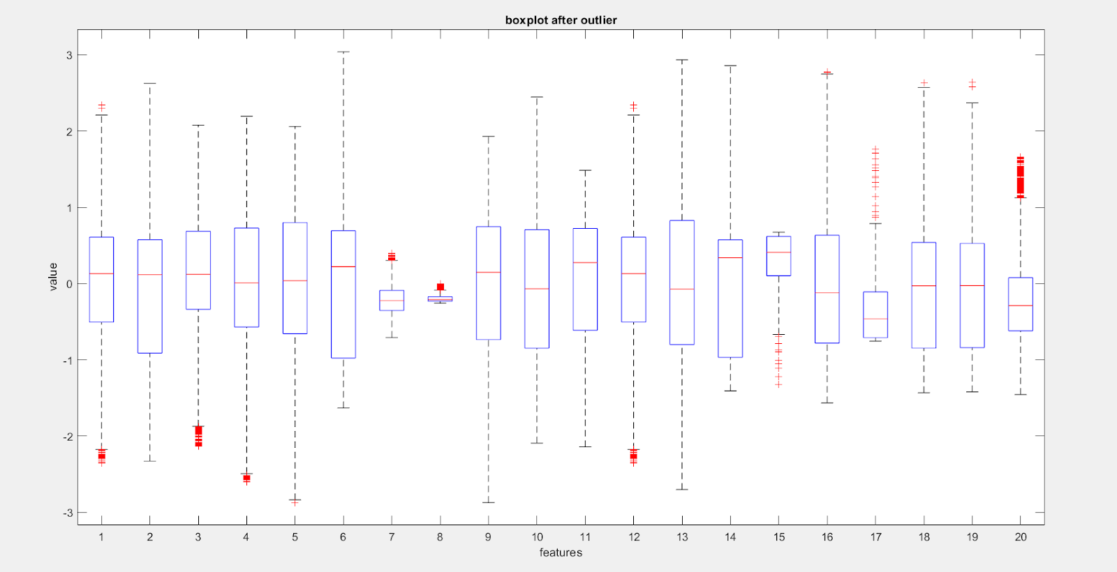
By comparison of number of red crosses present in the Fig 5 with the red crosses present in Fig 6 we can clearly observe that lot of outliers (in features) have been taken care of, but some outliers are still present in Fig 6,which are restricted to a small number of features and are heavily concentrated near the boundary of the outlier removal.

Here employing univariate method for detecting outlier such as IQR(box plot) as used above is not a right practice since the data is multivariate and we may be losing some valuable information. The data point which may seem like an outlier when just looking at univariate feature may actually not be an outlier when seen in n-dimensional plane where ‘n’ is the number of features.

Clustering analysis and outlier detection:

K-means clustering is a type of unsupervised learning which is used to find groups which have not been explicitly labeled in the data.The goal of this algorithm is to find groups in the data, with the number of groups represented by the variable K. The algorithm works iteratively to assign each data point to one of K groups based on the features that are provided. Data points are clustered based on feature similarity[16]. The results of the K-means clustering algorithm are:

1. The centroids of the K clusters, which can be used to label new data
2. Labels for the training data (each data point is assigned to a single cluster)

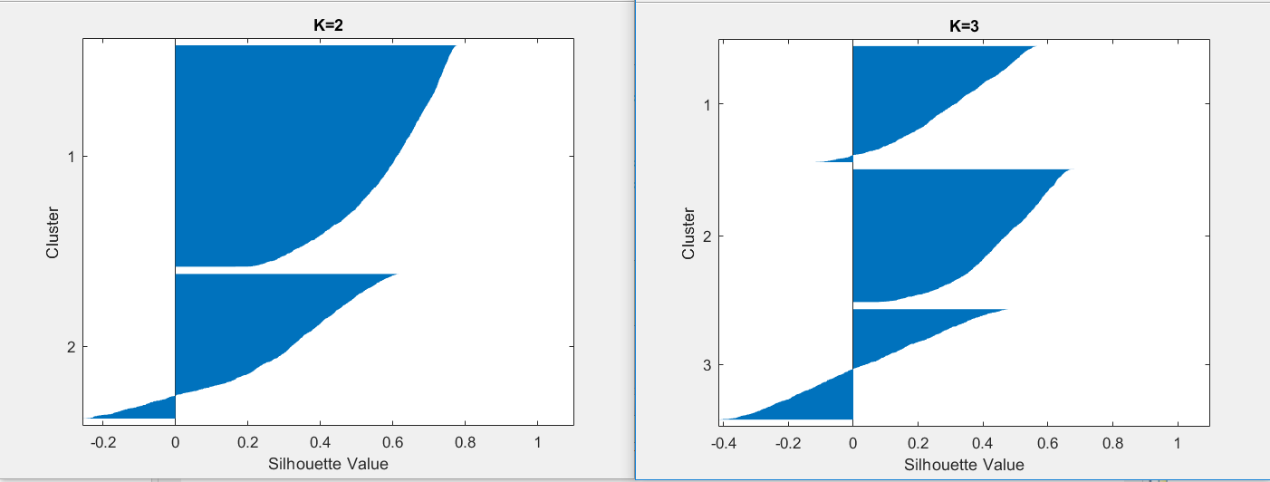
Rather than defining groups before looking at the data, clustering allows one to find and analyze the groups that have formed organically. It helps in identifying unknown groups in complex data set. Once the algorithm has been run and the groups are defined, any new data can be easily assigned to the correct group. This is a versatile algorithm that can be used for any type of grouping. To find the number of clusters in the data, the user needs to run the K-means clustering algorithm for a range of K values and compare the results. A commonly used method to compare results across different values of K is the mean distance between data points and their cluster centroid. Mean distance to the centroid as a function of K is plotted and the “elbow point,” where the rate of decrease sharply shifts and then does not change much, it can be used to roughly determine K. Here K=2 seems to be the right choice.The silhouette method may also be used for validating K.To get an idea of how well-separated the resulting clusters are, one can make a silhouette plot using the cluster indices output from kmeans. The silhouette plot displays a measure of how close each point in one cluster is to points in the neighboring clusters. This measure ranges from +1, indicating points that are very distant from neighboring clusters, through 0, indicating points that are not distinctly in one cluster or another, to -1, indicating points that are probably assigned to the wrong cluster. Average silhouette value for k=2 is 0.4599 and that for k=3 is 0.2774. Therefore K=2 is the choice for the number of clusters. This clustering method is also used for finding outliers in the dataset. The points which are very far located in the cluster may be considered as outlier. We are getting 72 outliers using this clustering method.

DATA SPLIT

We first randomly shuffle the data and then split the dataset into three parts:70% as training data, 15% of data for cross validation and remaining 15% as testing data. Training set is used to train a model, basically testing different algorithms and finding the best model to predict the outcomes then this model is applied on the cross validation dataset for tuning it before finalizing it for final testing, through this process we can improve the efficiency of the model by adjusting the trained model based on our observation and results we get for better accuracy and the testing set, fixed for the final testing of the most optimal algorithm, remained unused until that step. In cross validation lower K is usually cheaper and more biased. Larger K is more expensive, less biased, but can suffer from large variability. This is often cited with the conclusion to use k=10 [18].

Models

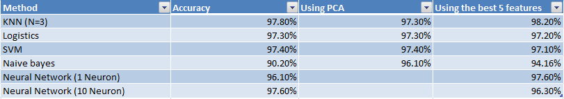
We propose to train the conventional models to learn the task of classifying male and female voice samples. The models we chose are as follows:

1. Logistic Regression
2. K Nearest Neighbors
3. Naive Bayes
4. Linear SVM
5. Neural Network

Full Feature Set We trained all the models mentioned above on the dataset containing all the 20 features.

Handpicking Top features We have picked the top five features analyzed in Important Feature section above.

Reducing Dimensionality by using PCA Reducing the dimensionality by using the PCA with variance 95%, with data reducing to 10 features.

PCA

Principal Component Analysis (PCA) is a technique in which correlations are found in features and the top performing features are extracted by applying orthogonal transformation on linearly uncorrelated variables called ’Principal Components’. PCA actually selects a linear combination of features and uses them as the new features. These new features can then be used to train the models. The number of principal components will depend upon the threshold of eigenvalues. Here, by taking 12 principal components we are able to get a variance in data greater than 0.95 (on a scale of 0 to 1) and the prediction accuracy of about 96 to 97 % for KNN classifier (sensitivity:0.984,specificity:0.95). It has been used to reduce dimensionality and to avoid redundancy in data.

Classification Models

Logistic Regression

It’s is a machine learning algorithm for classification. In this algorithm, the probabilities describing the possible outcomes of a single trial are modelled using a logistic function. Compared with other classification algorithms, it is more robust: the independent variables do not have to be normally distributed, or have equal variance in each group.In our model, we used 10 fold cross validation to seek out the optimal parameters.

KNN

KNN is an instance-based learning, where the function is only approximated locally and all computations are deferred until classification. It calculates the biggest number of the label of a data point’s K-Nearest Neighbor and assigns the point’s label as the biggest number one. KNN is effective when using a large-size of data and it is robust to outliers. Here we have taken k=3, since at this value of k we are getting optimum result.[20]

Naive Bayes Classifier

It is a classification technique based on Bayes Theorem with an assumption of independence among predictors. In simple terms, a Naive Bayes classifier assumes that the presence of a particular feature in a class is unrelated to the presence of any other feature. Even if these features depend on each other or upon the existence of the other features, all of these properties independently contribute to the probability.

SVM

In SVM, we solve an optimization problem i.e. to maximize the minimum distance of support vectors from the separator. We have a budget which allows the data to be misclassified i.e. on wrong side of the margin or hyperplane/separator. We have a constraint that prohibits on the number of misclassifications. This is called normalizing the betas or budget constraint. In our code, the first thing that clicks mind here now is using SVM with linear and radial basis function kernels[21]. We use cross validation to identify the penalty (lambda), for the misclassifications. We performed 10 fold cross validation to identify the best lambda. This lambda is identified by the cost parameter of box function taken as 1 identified using radial basis function.[19]

Neural Network

A neural network consists of units (neurons), arranged in layers, which convert an input vector into some output. Each unit takes an input, applies a (often nonlinear) function to it and then passes the output on to the next layer. Generally the networks are defined to be feed-forward: a unit feeds its output to all the units on the next layer, but there is no feedback to the previous layer. Weightings are applied to the signals passing from one unit to another, and it is these weightings which are tuned in the training phase to adapt a neural network to the particular problem at hand.[17]

CONCLUSION

Our dataset is balanced one with no missing value. It neither has high bias problem nor high variance problem. It is separable using a linear decision boundary.Each technique applied by us gave us good result, we consider there performance to be highly satisfactory.We have also performed Feature selection in our dataset, basically it is different from dimensionality reduction. Both methods seek to reduce the number of attributes in the dataset, but a dimensionality reduction method do so by creating new combinations of attributes, where as feature selection exclude attributes present in the data. Feature selection methods can be used to identify and remove irrelevant and redundant attributes from data that do not contribute to the accuracy of a predictive model. However, feature selection may cause some loss of information, as a result accuracy may somewhat reduce. Among all data preprocessing techniques applied we found Z score to be optimum for normalization, as it not only does mean normalisation but also scales the data which is essential in scale sensitive algorithms like KNN,PCA etc. Certain redundancy is observed in the features, to get rid of this PCA has been used which reduces the dimension, by giving uncorrelated principal components. Here the dimensionality is reduced without compromising much on the accuracy.

It has also been observed that the outliers removal leads to loss of data which can worsen the dataset on which it has been applied. So outliers removal is like a double edged sword which can either improve or worsen the dataset. Therefore, careful examination is required before labelling any data point as an outlier. We have applied multivariate outlier removal techniques like chi-square and Mahalanobis distance for reasons mentioned earlier (in outlier section). It is strongly felt that better & cleaner dataset beats the fancier algorithm.

Applying various algorithms we get the following results:

REFERENCES

1. https://www.kaggle.com/primaryobjects/voicegender

2. Gender Recognition using Voice by Vineet Ahirkar, Naveen Bansal, CS, UMBC,1000 Hilltop Cir, Baltimore, MD 21250,Copyright c 2017, Association for the Advancement of Artificial Intelligence (www.aaai.org)

3. Understanding Machine Learning: From Theory to Algorithms by Shai Shalev-Shwartz and Shai Ben-David

4. James Gareth, Daniela Witten, and Trevor Hastie. “An Introduction to Statistical Learning: With Applications in R.” (2014)

5. Shiming Xiang, Feiping Nie, Changshui Zhang, Learning a Mahalanobis distance metric for data clustering and classification

6. Data Mining-Concepts and Techniques(Authors: Jiawei Han Micheline Kamber Jian Pei) -Book

7. Xuan Guorong, Chai Peiqi and Wu Minhui, “Bhattacharyya distance feature selection,” Proceedings of 13th International Conference on Pattern Recognition

8. Howard Hua Yang and John Moody, Data Visualization and Feature Selection: New Algorithms for Non Gaussian Data

9. I Guyon , A Elisseeff, An Introduction to Variable and Feature Selection ,Journal of Machine Learning Research

10. Improving k-means by outlier removal, ACM

11. https://www.sciencedirect.com/science/article/pii/S1532046411000037

12. http://stat.ethz.ch/education/semesters/ss2012/ams/slides/v2.2.pdf

13. RG Garrett, The chi-square plot: a tool for multivariate outlier recognition, Journal of Geochemical Exploration

14. J. Han, M. Kamber and J. Pei, Data Mining - Concepts and Techniques, 3rd ed., Amsterdam: Morgan Kaufmann Publishers, 2012.

15. Duarte Silva, A.P., Filzmoser, P. & Brito, P. Adv Data Anal Classif (2017). https://doi.org/10.1007/s11634-017-0305-y

16. Hautamäki, Ville & Drapkina, Svetlana & Kärkkäinen, Ismo & Kinnunen, Tomi & Fränti, Pasi. (2005). Improving K-Means by Outlier Removal. 3540. 978-987. 10.1007/11499145_99.

17. DE Rumelhart, GE Hinton, RJ Williams,Learning representations by back-propagating errors

18. A Study of Cross-Validation and Bootstrap for Accuracy Estimation and Model Selection- Ron Kohavi (1995)

19. V Vapnik ,C Cortes,Support-vector networks

20. T. Cover, P. Hart, Nearest neighbor pattern classification

21. A Comparison Study of Kernel Functions in the Support Vector Machine

22. MATLAB-documentation, scikit-learn documentation, medium.com , stanford machine learning course & resources.